How the matched-null test works

The problem: clustering always returns clusters

Give a clustering method a single smooth cloud of points and it will still return clusters. Model-selection criteria behave the same way: BIC, the bootstrap likelihood-ratio test, the gap statistic all pick some number of groups, and on data with skew or correlation they often pick several. So when an analysis reports that a dataset contains, say, four personality types, the number may describe the population, or it may describe only the shape of the data under that method. Nothing in the output tells you which.

The matched-null test separates the two by asking a single question: would a dataset with the same margins and the same correlations, but no types, have produced the same answer?

Constructing the matched null

We want a reference dataset that matches the real one in every respect that is not in question, and is empty of the one thing that is. Two things are not in question: every variable’s marginal distribution, with its skew, its bounds and its lumps at round numbers on a Likert scale, and the correlations among variables. Latent groups, the thing in question, must be absent by construction.

By Sklar’s theorem that separation is always available: any joint distribution factors into its own margins and a copula carrying the dependence between them. Here the margins are taken from the real data and the copula is Gaussian.

Write the data as columns $X_1, \dots, X_p$ with empirical margins $F_1, \dots, F_p$ and correlation matrix $C$. Draw $Z \sim \mathcal{N}(0, \Omega)$ with $\Omega$ tuned so the induced correlations match $C$, then send each column back through its own empirical quantile function, $Y_j = F_j^{-1}\!\big(\Phi(Z_j)\big)$. Read from the inside out, that asks which percentile the Gaussian draw sits at and returns the real data value at that percentile.

Three properties carry the argument. Each $Y_j$ has exactly the empirical distribution of $X_j$, since the twin reshuffles observed values and invents none, so no marginal test can separate the two. The correlation matrix of $Y$ matches $C$ to within sampling error. And the copula contributes no clustering of its own: the Gaussian dependence is smooth, with no islands or gaps, so as long as each margin is itself unimodal the twin contains no cluster structure by construction. That qualifier is doing real work and is not boilerplate. A margin that is already multimodal is copied into the twin along with everything else, and it can carry groups in on its own; the section What the test declines to answer is about exactly that case. Outside it, whatever your pipeline reports on the twin was manufactured by the pipeline.

Both claims are cheap to check, so the block below is run and its output shown.

library(matchednull)

set.seed(1)
x <- matrix(rnorm(400 * 3), 400, 3) %*%
  chol(matrix(c(1, .5, .3, .5, 1, .4, .3, .4, 1), 3, 3))

twin <- copula_null(x)
all(sort(twin[, 1]) == sort(x[, 1]))   # margins: identical
#> [1] TRUE
round(cor(x) - cor(twin), 2)           # correlations: close
#>      [,1]  [,2]  [,3]
#> [1,] 0.00  0.01  0.05
#> [2,] 0.01  0.00 -0.03
#> [3,] 0.05 -0.03  0.00

The test statistic

Let $T(\cdot)$ be your pipeline, wrapped as a function that returns one number, typically the selected number of clusters, but it can be any scalar measure of clustering strength. Compute the real statistic $t_0 = T(X)$, then generate $R$ twins and compute $t_1, \dots, t_R$ with $t_r = T(Y^{(r)})$. The one-sided $p$-value is

$$p \;=\; \frac{1 + \#\{\, r : t_r \ge t_0 \,\}}{R + 1}.$$

The verdict reads null-like when $t_0$ sits inside the interval the twins produce, and exceeds the null when the real data stand out. The null is defined at the level of the data, not the pipeline, so the same twins work for a $k$-means heuristic, a published typology’s exact workflow, or a mixture model.

matched_null_test(x, cluster_fn = function(d) mclust::Mclust(d, verbose = FALSE)$G, R = 200)

Positive controls: sensitivity to genuine types

A test that never fires is worthless: it must stay quiet on typeless data and fire when genuine types are present. Figure 1 plants real types of two kinds and raises the signal strength.

Figure 1. Positive controls. Signal strength is the within-component correlation in panel A and the separation between means, in standard deviations, in panel B. The grey shaded band is the 95% interval of the matched-null median k: a point is red (detected) when the real value exceeds the band and grey (null-like) when it falls inside.

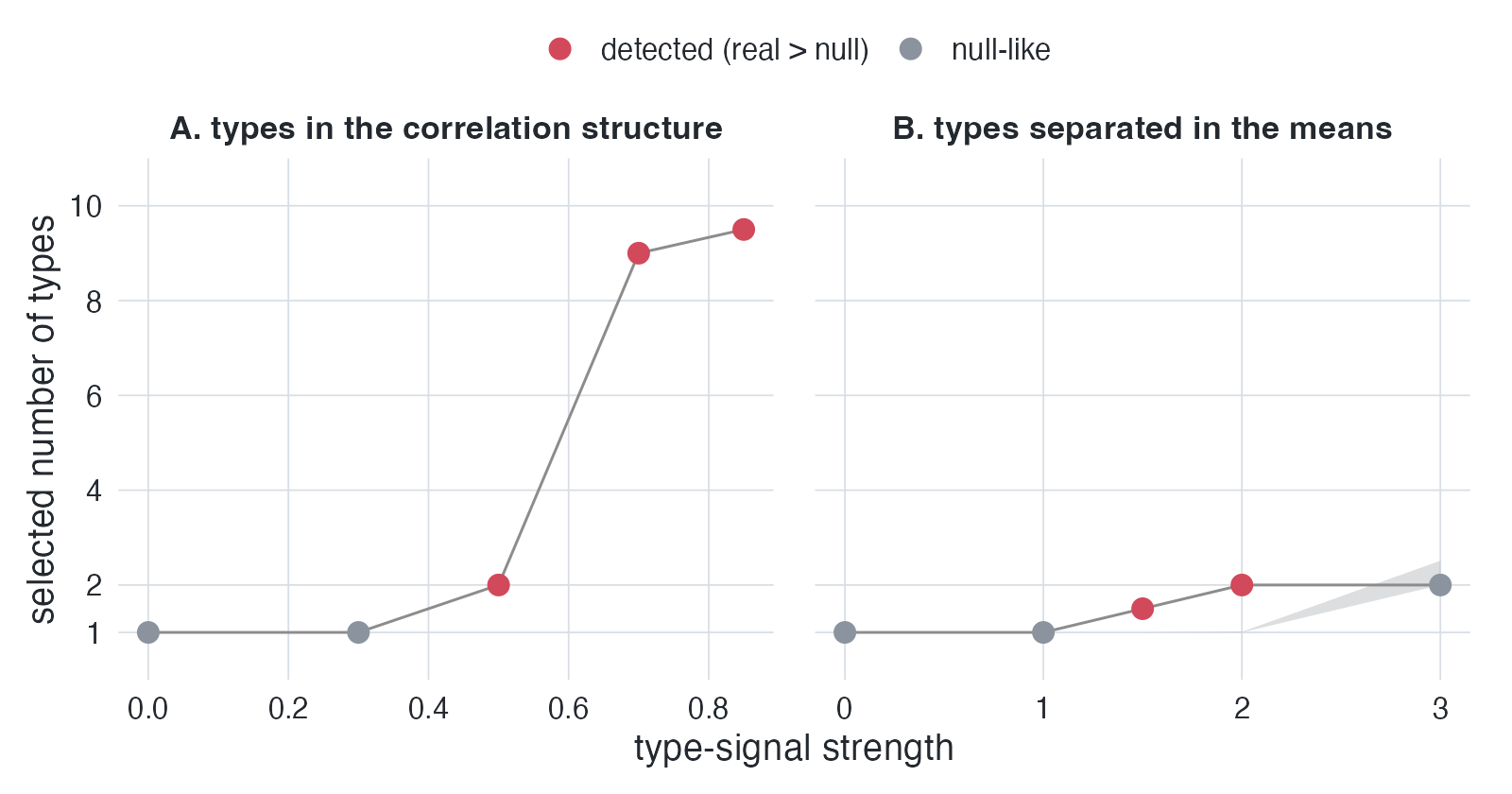
In panel A the types share identical margins and differ only in the orientation of their within-group correlations. A single Gaussian copula has one correlation matrix and cannot reproduce two, so as the within-group correlation grows the test fires. This is the regime that ordinary mean-comparison and marginal tests miss entirely: the groups are invisible one variable at a time and appear only in the joint dependence. In panel B the types are separated in their means in the familiar way, and the test fires there too as the separation grows, up to a point. At the largest separation it stops firing, which is not what a power curve is supposed to do, and that reversal is worth an explanation of its own; it gets one in What the test declines to answer. Setting that case aside for now, where there is structure the matched null cannot carry, the test finds it.

Empirical application: personality inventories

The motivating application is the claim that personality inventories contain a small number of latent “types.” Running the test across all fourteen mclust covariance parameterizations, on several public Big Five and HEXACO datasets, gives the specification curve in Figure 2.

Figure 2. Selected number of types across all fourteen mclust covariance models (steps), against the null band the twins produce (grey). The median verdict is null-like in every dataset.

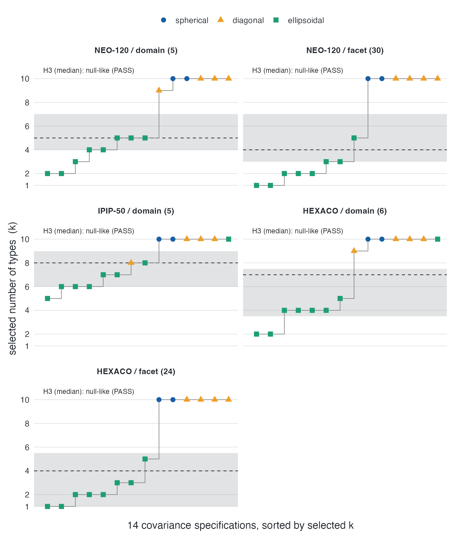
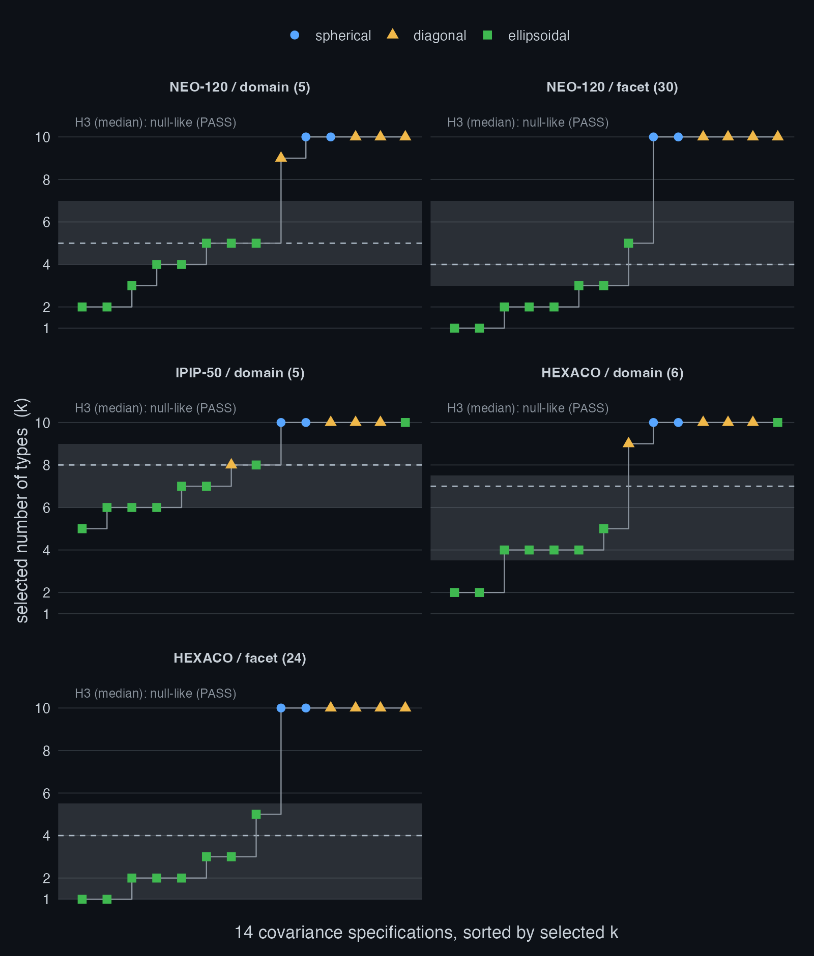
The number of types the pipeline selects (the step function) sits inside the band the twins produce (grey) for the great majority of specifications, and the median verdict is null-like in every dataset. The handful of specifications that climb above the band are the most flexible covariance models, which read the data’s skew and correlation as extra components; the twins, which share that skew and correlation, climb with them. The apparent “types” are the shape of the data under mclust, not latent kinds of people.

Convergent evidence from taxometrics

The mixture-model result lines up with an older tradition. The Comparison Curve Fit Index (CCFI) from taxometric analysis scores whether a construct is better described as categorical (taxonic) or continuous (dimensional), with values below the midpoint favouring a dimensional structure.

Figure 3. Comparison Curve Fit Index by trait for NEO-120 and HEXACO. Values fall on the dimensional side of the midpoint throughout.

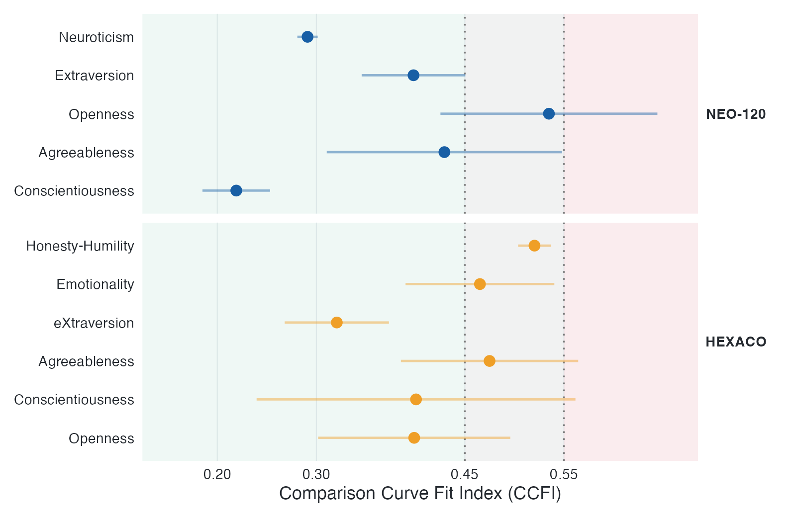
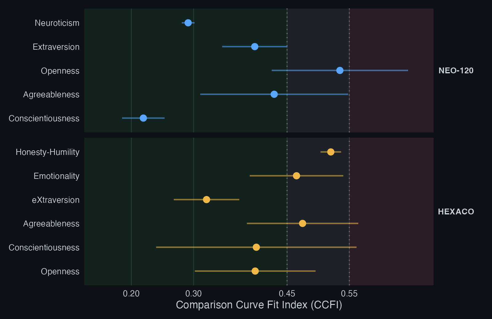
Every trait, in both inventories, falls on the dimensional side. Two methodological traditions that rarely meet, mixture-model cluster counting and taxometrics, return the same verdict, which is reassuring precisely because their assumptions differ.

A second, deliberately blinded null: the t-copula rung

The case for Gaussian minimality is made in full in the accompanying paper; this section takes it as given and asks what a second, tighter null adds.

The Gaussian copula is the null for this test, and it holds that position on purpose. Its dependence is exhausted by the correlation matrix, and among all distributions with a given covariance the multivariate normal has maximum entropy, so the twin carries the least structured dependence consistent with the data’s margins and correlations. A richer copula cannot take that role: a t copula adds tail dependence, a vine copula fits almost any dependence structure at all, and either would absorb into the null the very structure the test is meant to detect.

That absorption is what makes a t copula useful as a second null. Running one does not soften the test; it blinds the test, deliberately and in a known direction. An exceedance that survives a null which has already matched tail co-movement away cannot be attributed to tail co-movement. The Gaussian run remains the test. The t run is a follow-up question asked of an exceedance the Gaussian run has already licensed.

The question is worth asking because the failure mode has been measured. On typeless data whose dependence is non-Gaussian, generated from a t copula carrying tail dependence over a correlation matrix taken from real personality data, the count test fires in 99 to 100 percent of samples across tail-dependence strengths, as the accompanying paper reports. Standard criteria behave no better on the same data. Heavy-tailed dependence is not a rare edge case in questionnaire and clinical data, so a verdict of exceeds the Gaussian null does not on its own separate tails from types.

matched_null_test(x, cluster_fn, R = 200, copula = "t", df = 8)  # moderate tails
matched_null_test(x, cluster_fn, R = 200, copula = "t", df = 3)  # heavy tails

df sets how heavy the null’s tails are: smaller df means stronger tail co-movement, and as df grows the t null returns to the Gaussian one. The two values above bracket the range seen in questionnaire and clinical data, and both should be reported rather than the one that suits the conclusion. df is fixed by the user and never estimated from the sample. A null whose tail weight was fitted to the data would absorb tail structure adaptively, which is the failure this section exists to avoid.

The t rung never replaces the Gaussian run and is never reported alone. A matchednull result quoted without its Gaussian verdict is not a matched-null result.

Gaussian rung	t rung	Reading
not exceeded	not run	The count is what margins and correlations alone produce. Stop here; the t rung answers a question that has not arisen.
exceeded	exceeded	The exceedance is not attributable to tail co-movement. Proceed to the categorical-signature check.
exceeded	not exceeded	The exceedance was tail dependence, not types. Report it as such.
exceeded	mixed across df	Report the whole ladder, not the friendliest rung. Sensitivity to df is itself the finding.

Read the rungs in order. A lower rung that has not fired makes the rungs above it uninformative, not permissive.

The t rung and the categorical-signature check attack the same ambiguity from opposite directions. The t rung asks whether the exceedance survives once tail co-movement is matched away, which is a question about the null. The signature check, the taxometric evidence of the previous section, asks whether the structure carries the discontinuity a taxon would leave, which is a question about the data. They are independent, and a types claim needs both to agree. An exceedance that clears the t rung but shows no categorical signature is structure without evidence of kind; an exceedance the t rung reproduces is tail dependence whatever the signatures say.

Because the ladder is a sequence of tests, its rungs and its stopping rule belong in the preregistration alongside the summary statistic. Choosing which null to report after seeing the verdicts reintroduces the flexibility the matched null was built to remove. The conjunction rule used here, where a types claim requires exceedance at every rung run, is conservative by construction and needs no multiplicity correction. A disjunction rule, exceedance at any rung, would need one, and is not recommended.

What the test declines to answer

The t-copula check guards one way of misreading a verdict: the test fires, and what pushed it past the Gaussian twins was heavy tails, with no types involved. There is a second way, running in the opposite direction, where the test stays quiet even though real groups are present. It shows up inside the positive controls, which is the most awkward place for it to appear.

Go back to panel B of Figure 1, the one where the types are separated in their means. The test detects them at 1.5 and at 2 standard deviations of separation, and then, at 3 standard deviations, where the types are further apart than anywhere else in the figure, it goes quiet. Plotted as a power curve, it runs the wrong way. It cost me some time to be sure it was not a bug.

Follow the construction out to that end of the scale and the behaviour stops looking strange. By 3 standard deviations the two groups no longer hide in the joint dependence: each variable, taken by itself, has become visibly bimodal. The twin copies the observed values of every variable, so it copies that bimodal margin intact. And a bimodal margin is on its own enough to produce two components, with no help from the dependence structure at all. So the twin reports two clusters as well, the real value no longer stands out against the twins, and the verdict comes back null-like on a structure that is genuinely there. This is the case the qualifier in Constructing the matched null was pointing at.

It would be convenient to stop there and file the whole thing under expected behaviour, except that doing so skips the part worth examining, which is that the boundary follows from a choice, and the choice could have gone the other way. Preserving the observed margins exactly means conceding marginal shape to the null: whatever a single variable already displays becomes part of the reference, so it can never count as evidence. UNPaC (Helgeson, Vock, and Bair, 2021) makes the opposite choice, smoothing its margins to unimodality before building the reference, and on these same data it would report clustering. Under its own hypothesis it would be right to. Those are two different tests answering two different claims, and neither is a corrected version of the other.

What this narrows down to is a question smaller than “are there types,” and it is the same question the opening of this article already asked: would a dataset with the same margins and the same correlations, but no types, have produced this answer? Most of the time that smaller question is the one worth asking, since contested typologies rarely live in the margins to begin with. A variable that is plainly two-humped needs no copula null to reveal its groups; a histogram does it. Panel A is where the test earns its keep, because there every margin looks ordinary and the groups exist only in the joint dependence.

Since there is nothing here to repair, what the boundary leaves behind is a working habit. Inspect the margins for pronounced multimodality before you rely on the count test, and tie-break granular Likert-type scales before running formal unimodality tests. If a margin is visibly two-humped, this test is the wrong instrument for the question, and one of the methods in the next section may suit it better.

Related approaches

Testing a clustering result against a reference distribution is an old idea, and the choice of reference is what separates the methods.

The gap statistic (Tibshirani, Walther, and Hastie, 2001) compares the observed within-cluster dispersion to a uniform or PCA-aligned reference, which ignores the correlation structure of the data. SigClust (Liu, Hayes, Nobel, and Marron, 2008) tests a single two-way split against a single Gaussian null. Neither preserves the marginal distributions, which matters for the skewed and granular scales common in questionnaire data.

The closest relative is UNPaC (Helgeson, Vock, and Bair, 2021), which also builds its reference with a Gaussian copula. Its margins are the difference, as the previous section described: UNPaC smooths them to unimodality by kernel density estimation, so it keeps the power this test gives up. A second difference is in what gets compared. UNPaC evaluates a fixed cluster index, while matched_null_test() takes whatever scalar the user’s own pipeline returns, which is what allows a published typology’s exact workflow to be tested as it was actually run.

They complement each other. A result that clears the unimodal reference of UNPaC and the margin-preserving reference here is supported on both readings.

References

The method, its positive controls, and its false-positive calibration are described in the accompanying paper, Types Without Taxa: A Covariance-Matched-Null Multiverse Test of Categorical versus Continuous Personality Structure (Meng, 2026; preregistration: https://doi.org/10.17605/OSF.IO/2EKCG).

Helgeson, E. S., Vock, D. M., and Bair, E. (2021). Nonparametric cluster significance testing with reference to a unimodal null distribution. Biometrics, 77(4), 1215-1226. https://doi.org/10.1111/biom.13376

Liu, Y., Hayes, D. N., Nobel, A., and Marron, J. S. (2008). Statistical significance of clustering for high-dimension, low-sample size data. Journal of the American Statistical Association, 103(483), 1281-1293. https://doi.org/10.1198/016214508000000454

Tibshirani, R., Walther, G., and Hastie, T. (2001). Estimating the number of clusters in a data set via the gap statistic. Journal of the Royal Statistical Society Series B, 63(2), 411-423. https://doi.org/10.1111/1467-9868.00293