---
title: "Democracy, Crime, and Equity in the U.S. States"
subtitle: "Does state democratic backsliding track racial inequality in incarceration, and can felon re-enfranchisement undo it?"
author: "Miura Meng"
date: today
abstract: |
This report asks whether the health of state democracy is related to racial inequality in
incarceration across the United States, and whether one concrete reform, restoring the vote to
people with felony convictions, changes who turns out to vote. It draws on three public data
sources: the State Democracy Index 2.0, the Vera Institute's incarceration records, and a natural
experiment in Florida. The analysis proceeds in four steps, and each step revises the answer the
previous one seemed to give. A cross-sectional look suggests that more democratic states have
wider racial disparities, but that result is an artifact of the chosen measure: the Black/White
incarceration ratio is higher in those states only because they imprison far fewer white people.
Following each state over time instead, stronger democracy coincides with lower incarceration of
both groups, although a nationwide decline is the larger force. Grouping states by their joint
trajectories shows that the states which became more democratic decarcerated the most, while
those that backslid did so least. Finally, Florida's 2018 Amendment 4, the largest restoration of
felon voting rights in modern U.S. history, produced no measurable change in turnout, because a
follow-up law (SB7066) first required people to pay outstanding court fines. Again and again, careful
choices about measurement and design overturn the convenient story, and that is the report's
central point. Methodologically it applies mixed models,
group-based trajectory modeling, and synthetic control.
format:
html:
toc: true
toc-depth: 2
number-sections: true
embed-resources: true
theme: cosmo
code-fold: true
code-tools: true
df-print: kable
fig-align: center
execute:
warning: false
message: false
echo: true
---
```{r setup}
#| include: false
library(dplyr); library(tidyr); library(lme4); library(knitr)
proj <- ".."
df <- readRDS(file.path(proj, "data", "state_dem_incarceration.rds"))
```
# Question and contribution
Democracy, crime, and inequality all meet in one place: the criminal justice system. Democratic
institutions decide who writes the rules and whether power stays in check. The justice system is
where those rules reach individual people. Inequality, stated in statistical terms, is a difference
in how the same system treats different groups. Put together, these three give one question. Is the
health of a state's democracy related to racial inequality in its prisons, and can a democratic
reform change behavior on the ground?
The honest answer depends almost entirely on how the question is asked, and that dependence is the
report's real subject. I proceed in four steps, each one testing and then revising the conclusion
the step before it reached. The first measures inequality across states; the result looks alarming,
and a closer comparison takes the alarm apart. The second tracks each state against itself over
time, which dissolves that result and leaves a smaller signal worth trusting. The third asks whether
states sort into trajectory types; they do, loosely, though the method reads in more order than the
data really hold. The fourth turns to a natural experiment, the single point where cause can be
tested directly. Read in order, the steps make one argument: the convenient cross-sectional story
does not survive careful measurement, the version that survives is modest, and the reform that
should have moved the numbers was undone by its own fine print. The contribution is methodological.
It shows how far the answer travels as the method improves, not a new fact about democracy and
crime.
# Data and measures
Because the whole argument turns on measurement, it is worth being explicit at the start about the
data and, above all, about what "inequality" will mean. The analysis combines three public
datasets, each measured at the state-year level.
| Source | Unit | Coverage | Used for |
|---|---|---|---|
| State Democracy Index 2.0 (Grumbach & Bitton, UC Berkeley) | state-year | 2000 to 2023 | `democracy`, a latent score of democratic performance (higher is more democratic) |
| Vera Institute, Incarceration Trends | state-year | race-specific prison rates, 1990 to 2022 | Black and white prison rates per 100,000 |
| UF Election Lab (M. McDonald), Turnout 1980 to 2022 | state-year | even years | VAP turnout and counts of disenfranchised felons |
The choice that matters most is how to measure racial inequity, because there is no single correct
definition and, as the next section shows, the available definitions point in opposite directions.
I therefore carry three of them side by side and compare them directly: the Black/White rate ratio,
the absolute Black rate, and the gap between the Black and white rates (per 100,000). As a
benchmark, the U.S. Black/White prison-rate ratio over 2000 to 2022 has a median of about 5.4,
which the dataset confirms below. With the data and these competing measures in place, the first
question is simply what a direct comparison across states reveals.
# Measurement decides the answer
Begin with the question in its most direct form. If I average each state over 2016 to 2020 and plot
the Black/White incarceration ratio against the State Democracy Index, more democratic states
appear to have wider racial disparities. Taken at face value this is a provocative result, since it
would imply that democratic health and racial fairness in punishment pull in opposite directions.
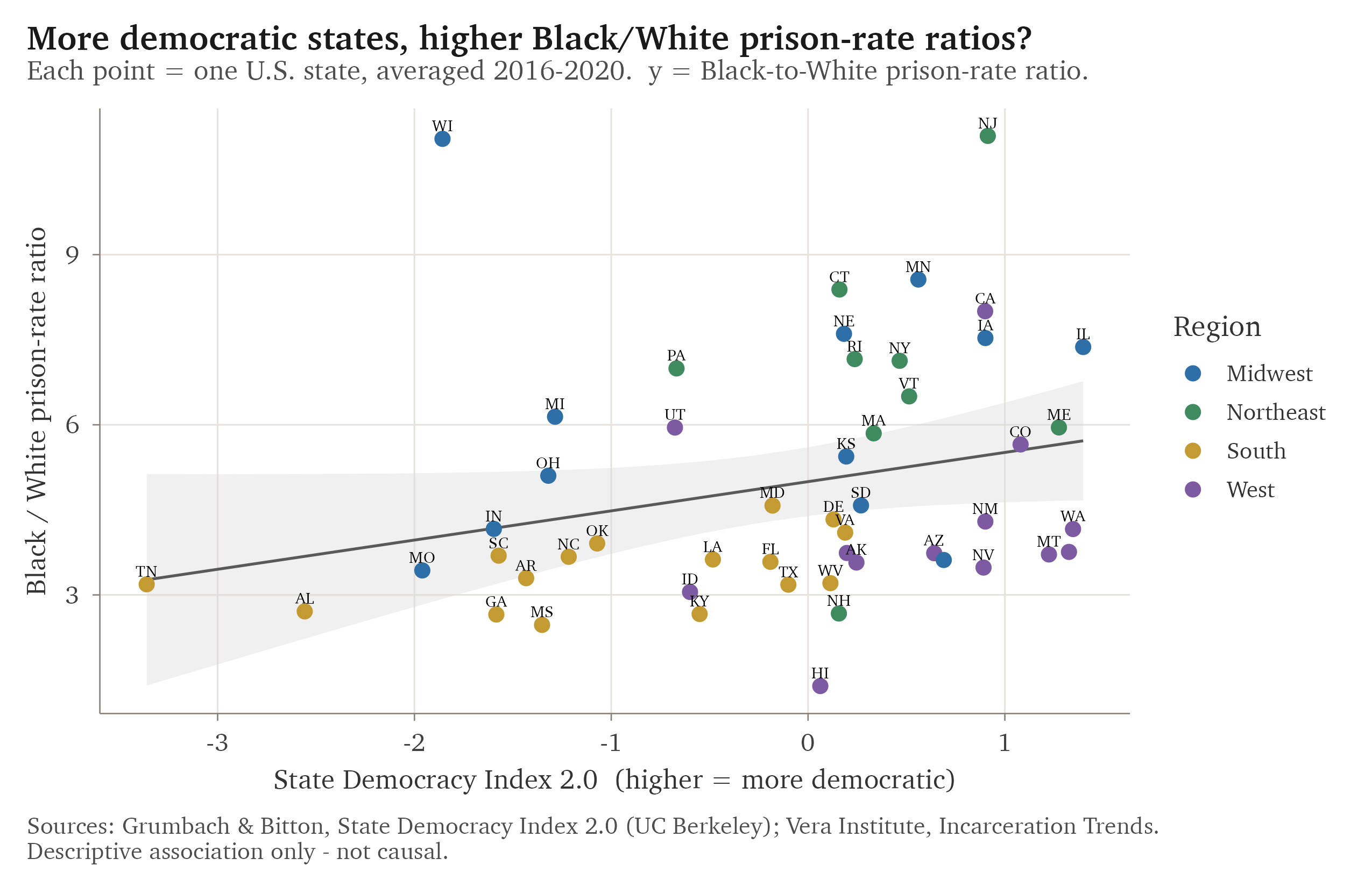
The result does not survive a change of measure. Here is why.
If I hold the democracy axis fixed and substitute four definitions of racial inequity, the
correlation does not merely weaken. It changes sign.
```{r equity-cor}
#| code-summary: "Recompute the four democracy and inequity correlations (2016 to 2020 cross-section)"
win <- 2016:2020
st <- df |>
  filter(year %in% win, is.finite(black_prison_pop_rate),
         is.finite(white_prison_pop_rate), is.finite(democracy)) |>
  group_by(state_abbr) |>
  summarise(democracy  = mean(democracy),
            black_rate = mean(black_prison_pop_rate),
            white_rate = mean(white_prison_pop_rate), .groups = "drop") |>
  mutate(bw_ratio = black_rate / white_rate, gap = black_rate - white_rate)
cors <- sapply(c("bw_ratio","black_rate","white_rate","gap"),
               function(v) cor(st$democracy, st[[v]]))
tibble(`Inequity measure` = c("Black / White ratio","Absolute Black rate",
                              "Absolute White rate","Gap (Black minus White)"),
       `Correlation with State Democracy Index` = round(cors, 2)) |>
  kable(align = "lc")
```
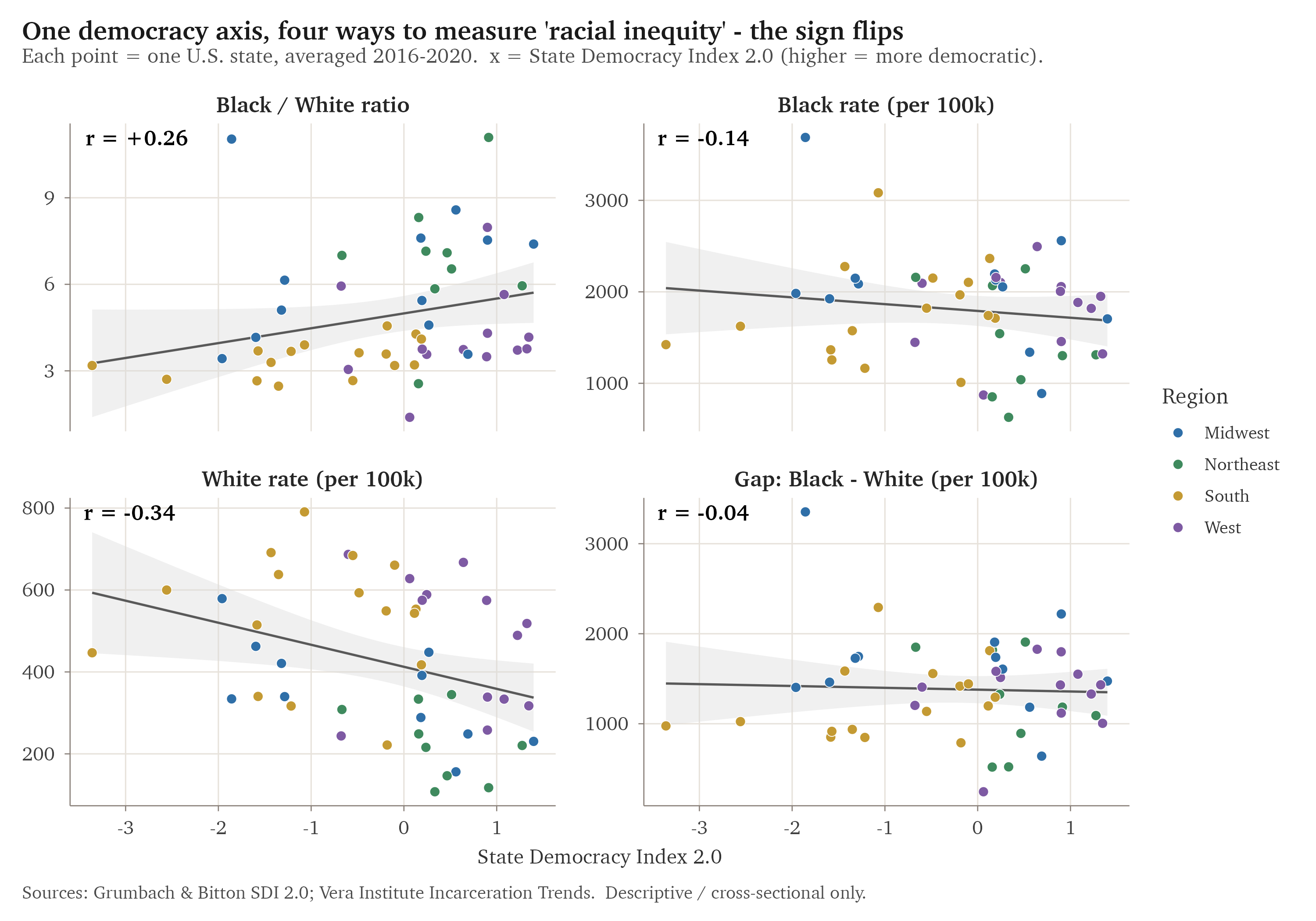
The mechanism is the white incarceration rate. More democratic states imprison far fewer white
people (a correlation of about -0.34), and because the ratio divides the Black rate by the white
rate, a smaller white rate inflates the ratio even when Black incarceration has not changed. The
South shows a lower ratio not because it punishes Black and white residents more equally, but
because it imprisons white residents at high rates too, which enlarges the denominator. Measured by
the absolute Black rate, more democratic states are if anything slightly better, and the absolute
gap is essentially flat. The number reported most often, the ratio, is also the one most likely to mislead: it can move for
reasons that have nothing to do with how Black residents are treated. And it has a direct methodological consequence. If a
single cross-section can be turned upside down by the choice of denominator, then comparing
different states is too weak an instrument for a question that sounds causal. The natural correction
is to stop comparing states with one another and start comparing each state with itself.
# Following each state over time
Comparing states with one another mixes democracy together with everything else that makes states
differ: region, demographics, history, and the local economy. The previous section showed how badly
that mixing can distort the answer. A cleaner question is longitudinal. When a given state's
democracy rises or falls, does its incarceration move with it? Because each state then serves as its
own control, the fixed differences that contaminated the cross-section drop out of the comparison.
To make this precise I split the democracy score into two parts. The first is each state's long-run
average, which carries the between-state variation that the earlier figures relied on. The second is
each year's deviation from that average, which carries the within-state variation that tracks change
over time. This within/between split follows Mundlak (1978). I then fit a linear mixed model with a
random intercept for each state and a common year trend, so that the two kinds of variation are
estimated side by side rather than confused with each other.
```{r within-between}
#| code-summary: "Fit the three within and between mixed models (lme4)"
panel <- df |>
  filter(is.finite(bw_ratio), black_prison_pop_rate > 0, white_prison_pop_rate > 0,
         is.finite(democracy)) |>
  group_by(state_abbr) |>
  mutate(dem_between = mean(democracy), dem_within = democracy - dem_between, n = n()) |>
  ungroup() |> filter(n >= 10) |> mutate(year_c = year - 2011)

outc <- c("log(Black/White ratio)" = "log(bw_ratio)",
          "log(Black rate)"        = "log(black_prison_pop_rate)",
          "log(White rate)"        = "log(white_prison_pop_rate)")
res <- lapply(names(outc), function(nm) {
  m  <- lmer(as.formula(paste0(outc[[nm]],
              " ~ dem_within + dem_between + year_c + (1 | state_abbr)")), data = panel)
  co <- summary(m)$coefficients
  tibble(Outcome = nm,
         `Within-state`  = round(co["dem_within","Estimate"], 3),
         `Between-state` = round(co["dem_between","Estimate"], 3),
         `Year trend`    = round(co["year_c","Estimate"], 3))
}) |> bind_rows()
kable(res, align = "lccc")
```
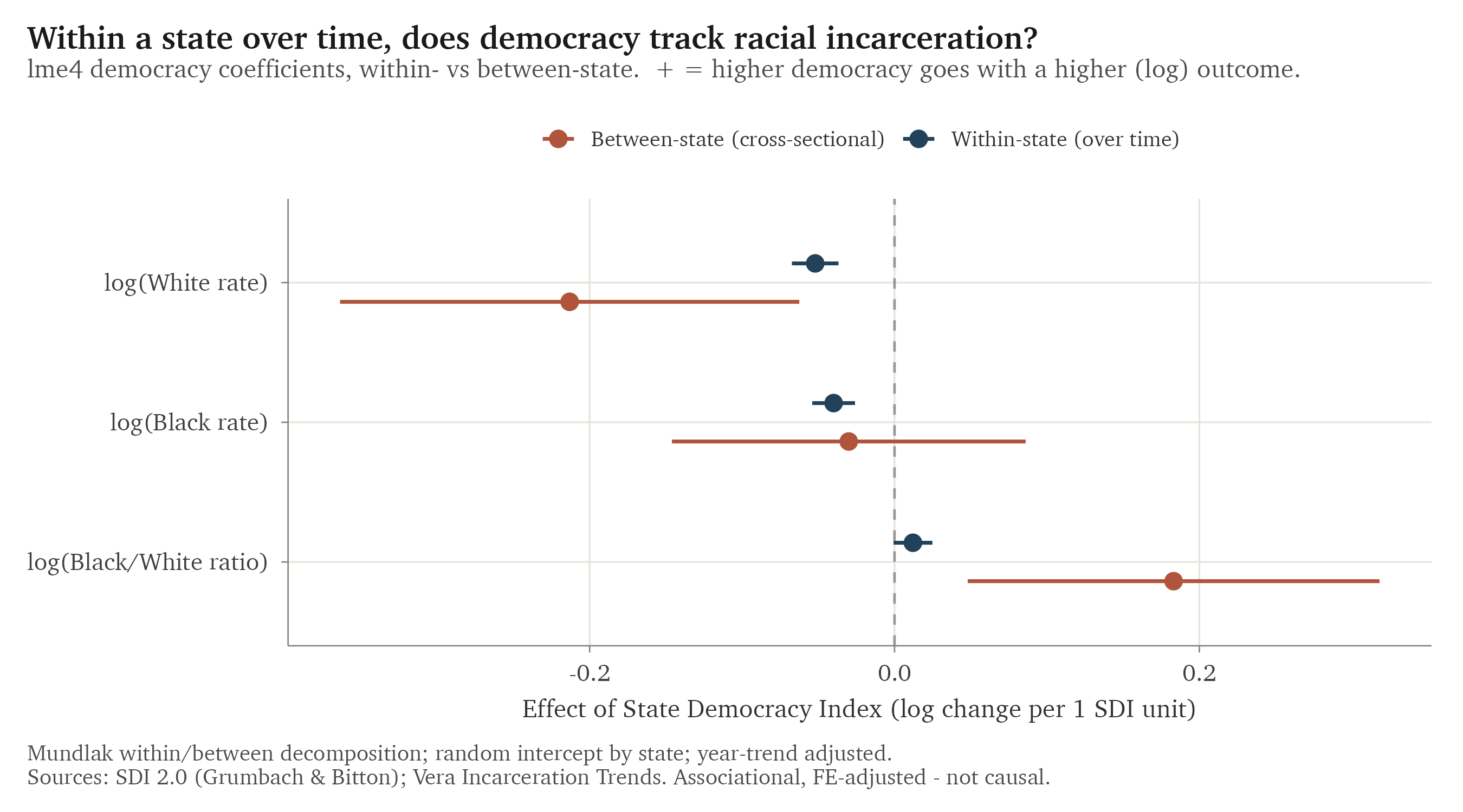
The table separates the signal from the artifact. The alarming cross-sectional result for the ratio
is entirely between-state (about +0.18) and vanishes within states (about +0.01), which means it
reflects which states are which rather than what happens when a state's democracy changes. Within
states, stronger democracy goes with lower incarceration of both groups, about -0.04 for the Black
rate and -0.05 for the white rate in log points per index unit. Because the two rates fall together,
the ratio barely moves, which is exactly what the measurement discussion predicted. The largest
term in every model, however, is neither within nor between democracy but the year trend: the ratio
fell about 2.6 percent a year and the Black rate about 2.7 percent a year. Most of the movement in
racial incarceration over this period is a nationwide decline that has little to do with state
democracy, and an analysis that left time out would mistake that tide for its own discovery. The
within-state association is consistent in direction and modest in size, and the argument is
stronger for saying so plainly.
# From multiverse to model
The heading marks a move. The first two steps were a small multiverse, one question carried through
choices that should not change the answer so the disagreements could show; this section turns that
multiverse into a single Bayesian model, in which the same choices reappear as contrasts of one
posterior. The multiverse is the better tool for revealing that the choices matter; the model is the
better tool for saying how much, and how reliably.
The first two steps treated the choice of measure and the choice of comparison as separate decisions.
They are not. The four measures and the within and between contrasts are all summaries of the same two
underlying quantities: how heavily a state imprisons its Black residents, how heavily it imprisons its
white residents, and how each of those moves with democracy. So rather than walk the choices one at a
time, I can fit a single model of those two quantities and read every choice off the one set of
estimates it implies.
The model carries two outcomes at once, the log Black rate and the log white rate, each depending on
democracy in the same within/between split as the previous section, with a random intercept for each
state and the two outcomes free to correlate. It is Bayesian, fit with brms, and it converged cleanly.
The coefficients are scaled per standard deviation of democracy, so they are not directly comparable in
size to the previous table, but their signs and pattern are the same.
```{r bayes-expansion}
#| code-summary: "Fit or load the joint Bayesian model and read the four measures off one posterior (brms)"
suppressMessages({library(brms); library(posterior)})
bd <- df |>
  filter(is.finite(black_prison_pop_rate), is.finite(white_prison_pop_rate),
         black_prison_pop_rate > 0, white_prison_pop_rate > 0, is.finite(democracy)) |>
  mutate(logB = log(black_prison_pop_rate), logW = log(white_prison_pop_rate)) |>
  group_by(state_abbr) |> mutate(demM_raw = mean(democracy)) |> ungroup() |>
  mutate(demW_raw = democracy - demM_raw, yearc = (year - 2011) / 10)
sm <- bd |> distinct(state_abbr, demM_raw)
bd$demM <- (bd$demM_raw - mean(sm$demM_raw)) / sd(sm$demM_raw)
bd$demW <- bd$demW_raw / sd(bd$demW_raw)
fit_path <- file.path(proj, "bayes_fit.rds")
if (file.exists(fit_path)) {
  fit <- readRDS(fit_path)
} else {
  fit <- brm(bf(logB ~ demW + demM + yearc + (1 | p | state_abbr)) +
             bf(logW ~ demW + demM + yearc + (1 | p | state_abbr)) + set_rescor(TRUE),
             data = bd,
             prior = c(prior(normal(0, 1), class = b, resp = "logB"),
                       prior(normal(0, 1), class = b, resp = "logW")),
             chains = 4, iter = 4000, warmup = 1000, seed = 20260620,
             cores = 4, refresh = 0, control = list(adapt_delta = 0.95))
  saveRDS(fit, fit_path)
}
dr <- as_draws_df(fit)
ci <- function(x) sprintf("%+.3f [%+.3f, %+.3f]", median(x), quantile(x, .025), quantile(x, .975))
Bb <- dr$b_logB_demM; Wb <- dr$b_logW_demM
Bw <- dr$b_logB_demW; Ww <- dr$b_logW_demW
tibble(
  Measure = c("Black/White ratio", "absolute Black rate", "absolute White rate"),
  `Between-state (per 1 SD)` = c(ci(Bb - Wb), ci(Bb), ci(Wb)),
  `Within-state (per 1 SD)`  = c(ci(Bw - Ww), ci(Bw), ci(Ww))
) |> kable(align = "lcc")
```
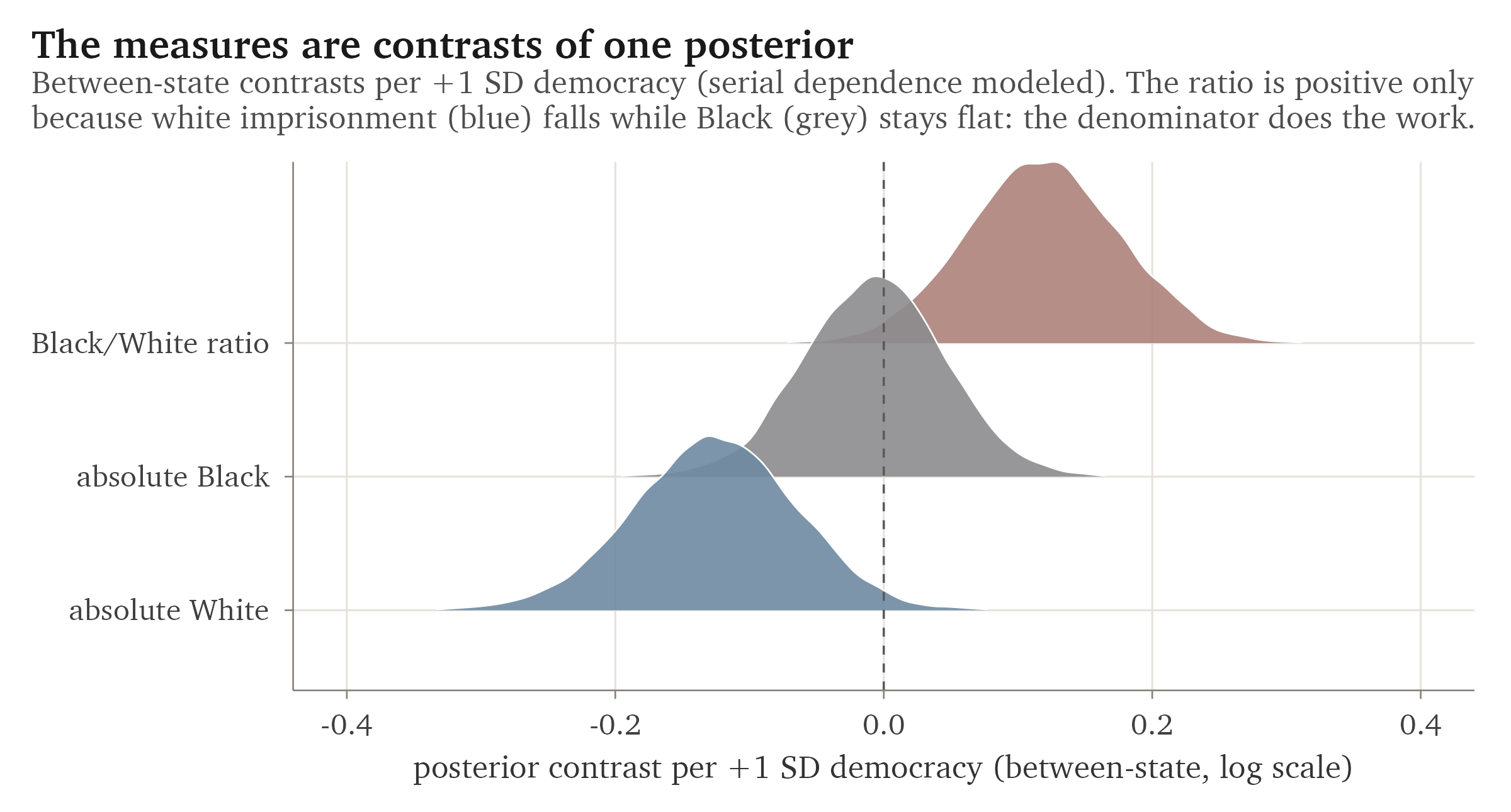
The table and the figure tell one story. Between states, stronger democracy goes with a much lower
white rate and a roughly flat Black rate, so the ratio, which is just their difference, comes out
positive: the alarming cross-sectional pattern is the white denominator again, now derived rather than
asserted. Within states the two rates fall together and the ratio barely moves. Because every number
comes from the same posterior, I can also ask how reliably the measures disagree. The probability that
democracy raises the ratio while leaving the white rate lower, the exact shape of the first step's
reversal, is about 0.99; the weaker claim, that the ratio rises while the absolute Black rate falls,
holds with probability about 0.68, lower only because the Black rate sits close to flat. The reversal
is a near-certain feature of how the two rates move, not a fragile accident of one comparison.
None of this is causal. The model rearranges the same observational evidence more economically; it does
not identify an effect. Its value is to show, in one place, that the disagreements among the measures
are not four findings but four sides of one model, and to put a number on how much each choice matters.
The code is in `R/08_bayes_expansion.R`.
One thing even this unified model cannot reveal is whether states resemble one another in how democracy
and punishment move together, or whether a single number hides very different state experiences. To see
that, we have to look at whole trajectories.
# A typology of state trajectories
An average coefficient describes the typical state but conceals the variation across states, and
that variation is itself part of the story. The question now is whether states sort into
recognizable types according to how democracy and incarceration evolved together. Group-based
trajectory modeling, a method developed in criminology by Nagin and Land (1993) to classify
offending over the life course, is built for this task. It sorts the fifty states by their joint
path from 2000 to 2022 on two measures at once, democracy and the logged Black incarceration rate.
The BIC selects five well-separated groups, with an average posterior probability of assignment near
0.99.
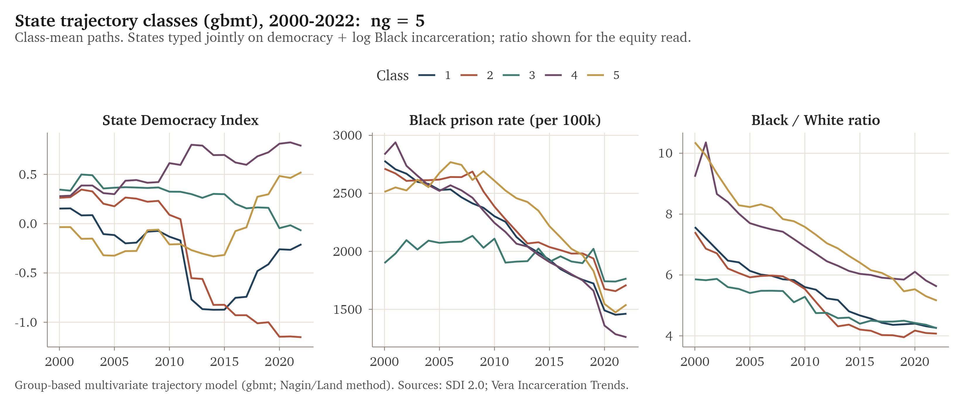
The classes line up along a single spectrum, which is what makes them interpretable rather than
arbitrary (means shown for 2000 and 2022).
| Class | Example states | Democracy | Black rate | Reading |
|---|---|---|---|---|
| 4 | CA, NY, NJ, MA, CT, WA | 0.28 → 0.79 | 2835 → 1260 | grew more democratic, decarcerated the most |
| 5 | FL, IL, PA, VA, MN | -0.04 → 0.52 | 2513 → 1541 | grew more democratic, ratio converged |
| 1 | GA, MD, MI, OH, TX | 0.15 → -0.21 | 2780 → 1462 | slight decline, still large decarceration |
| 3 | AR, ID, MT, NE, WV | 0.35 → -0.07 | 1899 → 1765 | stuck: the Black rate barely moved |
| 2 | AL, MS, TN, OK, WI | 0.26 → -1.15 | 2713 → 1710 | backslid the most; the white rate rose |
The pattern reinforces the within-state result and gives it a recognizable shape. States that grew
more democratic also reduced incarceration the most, and the states that backslid the furthest, the
group in Class 2 that Grumbach (2023) calls the laboratories of backsliding, reduced Black
incarceration the least and even saw their white rate rise. This is the same association as before,
now visible as a contrast between identifiable groups of states rather than as a single coefficient.
Three cautions keep the typology honest, and each one limits how much weight it can carry. Every
class reduced incarceration, because the national decline runs through all of them, so the groups
differ in degree rather than in direction. The ratio converged toward four or five everywhere, which
means that by that measure disparities narrowed across the board regardless of democracy. And
because the BIC keeps improving as more groups are added, the number of classes is not firmly pinned
down, and highly autocorrelated series like these can produce groups that are not really there. The
classes are useful summaries, not natural kinds, and they remain entangled with region. Most
important for the argument, a typology still only describes how things moved together. It cannot
show that democracy caused any of it. For that we need a moment when democracy itself was changed on
purpose.
# A causal test: Florida's Amendment 4
One state did exactly that. In 2018 Florida passed Amendment 4, which restored voting rights to roughly
1.4 million people with felony convictions, the largest single restoration in modern U.S. history.
Because the vote was expanded deliberately and all at once, Florida is one of the few places where
we can ask whether the expansion actually moved turnout, and not just whether turnout drifted the
same way on its own.
With a single treated state, I use synthetic control (Abadie, Diamond, and
Hainmueller, 2010). The method builds a "synthetic Florida" from a weighted combination of states
that did not change their felon-voting laws, chosen so that the combination reproduces Florida's
turnout history before the reform, and then reads the reform's effect as the gap that opens
afterward. I use VAP turnout as the outcome, because its denominator is the voting-age population
and therefore does not move mechanically when people are re-enfranchised. A placebo, or permutation,
test provides inference by asking how unusual Florida's gap is against the same gaps computed for
every donor state.
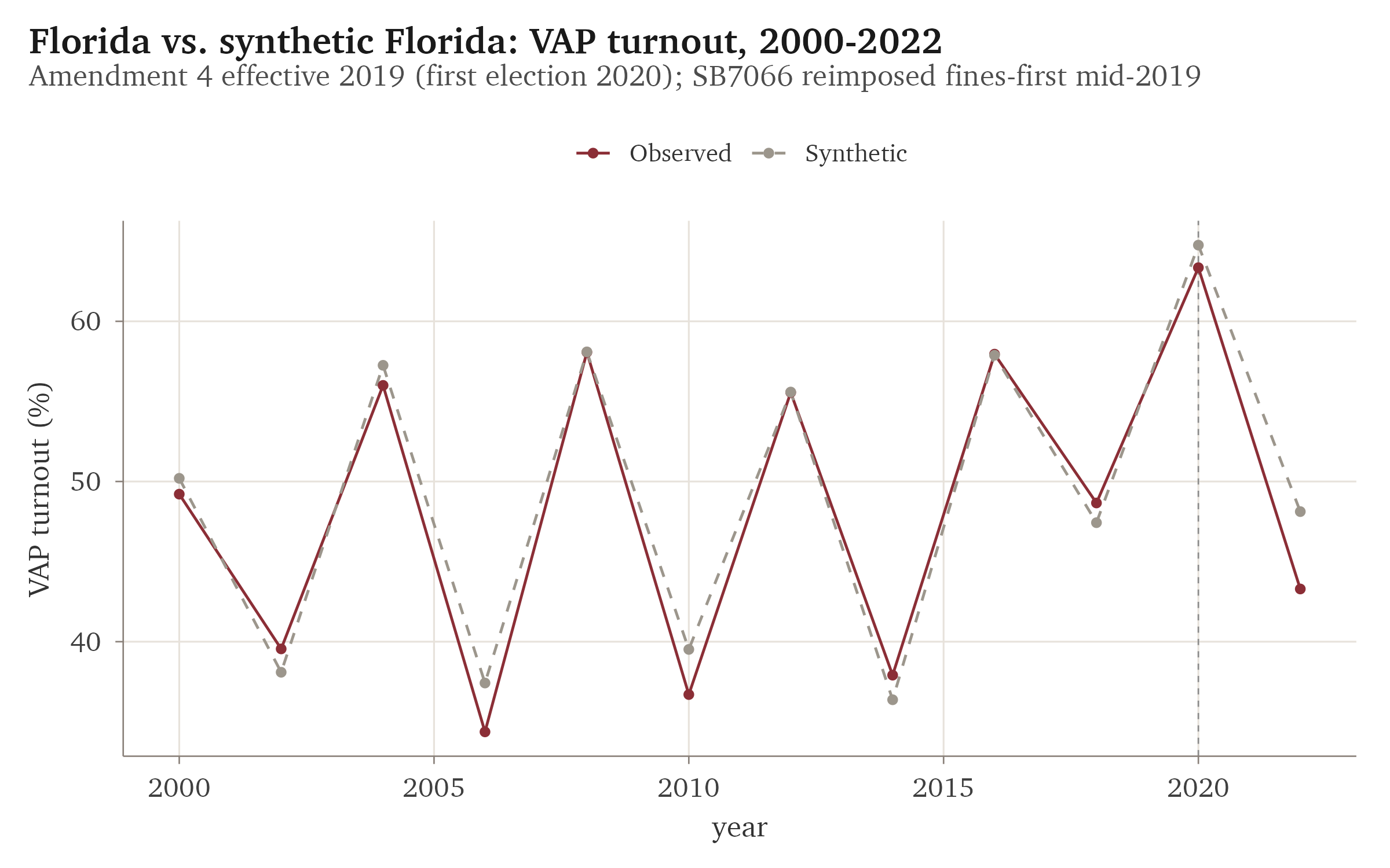
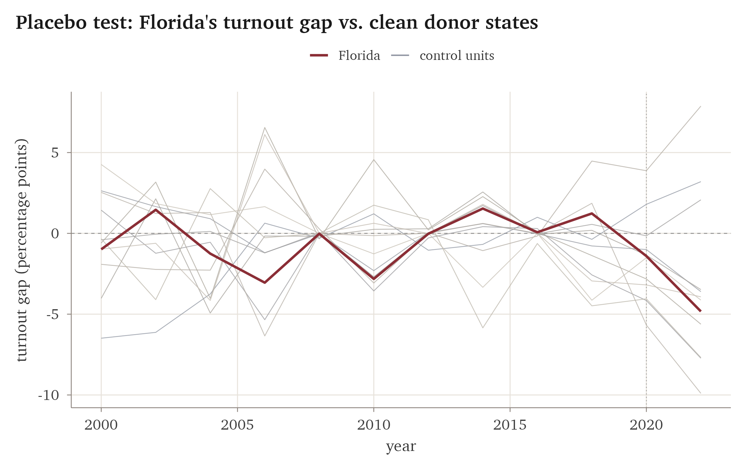
The pre-reform fit is close, with a 2016 gap of only 0.07 points, which gives the comparison
credibility. After the reform the gaps are -1.4 points in 2020 and -4.8 in 2022, both negative
rather than positive, and the placebo test returns a p-value of about 0.14, which means Florida is
not unusual among the donor states. Amendment 4 produced no detectable increase in turnout.
A null result is only worth reporting if we can say why it happened, and here the reason is visible
in the same data. The reform barely took effect. Florida's disenfranchised share fell only from
1.25 percent of the voting-age population in 2018 to 1.16 percent in 2020 and 1.14 percent in 2022,
a nearly flat line rather than the steep drop that re-enfranchising 1.4 million people would imply.
The explanation is that a second law passed in mid-2019, SB7066, required people to pay all
outstanding court fines and fees before regaining the vote. That payment requirement works as a
wealth test on the franchise, and it falls hardest on poor and disproportionately Black Floridians.
The null is itself the story: a democratic expansion
was largely cancelled by a second, regressive measure before it could change behavior. This is the
cleanest causal statement the report can make, and it ties back to where the earlier sections began.
The cross-section offered a link that turned out to be an artifact; the within-state and trajectory
analyses offered a small one. The single deliberate intervention available to test shows that even a
large, direct expansion of democratic rights can come to little once its implementation is undone.
# Limitations
The argument depends on taking each step's weaknesses seriously, so the main ones belong in the open
rather than in a footnote.
Aggregate turnout is a blunt instrument. Even a fully effective Amendment 4 (about 8 percent of the
voting-age population, most of whom never register or vote) might move statewide turnout by less than
one point, below what this design can detect. The null says the effect was too small for this test to see, not that re-enfranchisement does
nothing. A finer test would follow the formerly incarcerated themselves through the voter files.
The first three sections are observational. The mixed models adjust for fixed differences between
states, but they still cannot show that democracy causes anything, and the trajectory classes only
describe how groups of states moved, region and all. So these sections help frame the question. They
do not answer it.
State democracy and incarceration are themselves estimated quantities. A fuller treatment would
compare alternative measures and carry the resulting estimation error through the analysis.
The synthetic control rests on a single treated state, an imperfect pre-period fit in midterm years,
a small pool of clean donor states that limits statistical power, and a 2020 treatment year that
coincided with the pandemic turnout surge. The placebo p-value should be read with that limited
power in mind.
# What this adds, and what comes next
The four steps make one argument, and it is worth stating plainly. The relationship between state
democracy and racial inequality in incarceration is weaker and far more measurement-dependent than a
single cross-section suggests. The ratio that is reported most often points the wrong way for a
mechanical reason. The credible link, visible only within states over time, is small beside
a national decline in incarceration. And the one reform clean enough to test causally left no mark on
turnout because a second law neutralized it. None of these is a breakthrough on its own. Together
they make a more useful point: on a question like this the method carries the
finding, and disciplined measurement and design repeatedly overturn the convenient answer.
That habit is what the analysis is meant to show, and the whole pipeline is reproducible from
raw data to figures.
Three extensions would sharpen the argument, each aimed at the weakest link above. Individual
voter-file data would give a far more sensitive test of Amendment 4 than aggregate turnout, by
following the formerly incarcerated themselves rather than the entire electorate. A staggered design
across the many states that changed felon-voting rules between 2016 and 2022 would turn a single case
into many and improve both statistical power and external validity. And alternative trajectory
estimators with bootstrap resampling would show how firm the five-class typology really is. Each of
these tightens a claim I deliberately kept cautious.
# References
## Data sources
Grumbach, J. M., & Bitton, F. (2024). *State Democracy Index 2.0* [Data set]. Democracy Policy Lab, University of California, Berkeley. <https://democracypolicylab.berkeley.edu/state-democracy-index/>
McDonald, M. P. (2023). *United States Elections Project: Voter Turnout Data, 1980–2022* [Data set]. UF Election Lab, University of Florida. <https://election.lab.ufl.edu/voter-turnout/>
Vera Institute of Justice. (2024). *Incarceration Trends* [Data set]. <https://github.com/vera-institute/incarceration-trends>
## Methods and software
Abadie, A., Diamond, A., & Hainmueller, J. (2010). Synthetic Control Methods for Comparative Case Studies: Estimating the Effect of California's Tobacco Control Program. *Journal of the American Statistical Association, 105*(490), 493–505.
Bates, D., Mächler, M., Bolker, B., & Walker, S. (2015). Fitting Linear Mixed-Effects Models Using lme4. *Journal of Statistical Software, 67*(1), 1–48.
Dunford, E. (2023). *tidysynth: A Tidy Implementation of the Synthetic Control Method* [R package]. <https://CRAN.R-project.org/package=tidysynth>
Magrini, A. (2022). *gbmt: Group-Based Multivariate Trajectory Modeling* [R package]. <https://CRAN.R-project.org/package=gbmt>
Mundlak, Y. (1978). On the Pooling of Time Series and Cross Section Data. *Econometrica, 46*(1), 69–85.
Nagin, D. S., & Land, K. C. (1993). Age, Criminal Careers, and Population Heterogeneity: Specification and Estimation of a Nonparametric, Mixed Poisson Model. *Criminology, 31*(3), 327–362.
R Core Team. (2025). *R: A Language and Environment for Statistical Computing* (version 4.5.2). R Foundation for Statistical Computing. <https://www.R-project.org/>
## Policy and other works
Florida Department of State, Division of Elections. (2018). *Amendment 4: Voting Restoration Amendment* (Florida Constitution, Art. VI, § 4).
Florida Legislature. (2019). *Senate Bill 7066.*
Grumbach, J. M. (2022). *Laboratories against Democracy: How National Parties Transformed State Politics*. Princeton University Press.
Grumbach, J. M. (2023). Laboratories of Democratic Backsliding. *American Political Science Review, 117*(3), 967–984.
The Sentencing Project. (2024). *Locked Out 2024: Four Million Denied Voting Rights Due to a Felony Conviction.*
# Reproducibility {.appendix}
Every figure and all modeling results in this report are produced by the scripts in `R/`, run in order; a few descriptive summary statistics quoted in the text are computed directly from the source data. All
analyses use R (R Core Team, 2025) with the packages lme4 (Bates et al., 2015), gbmt (Magrini,
2022), and tidysynth (Dunford, 2023).
| Script | Produces |
|---|---|
| `01_load_merge.R` | the merged state-year dataset (`data/state_dem_incarceration.rds`) |
| `02_first_plot.R` | cross-section of democracy against the Black/White ratio |
| `03_equity_measures.R` | the four-measure comparison |
| `04_within_state_models.R` | the within and between mixed models, with figure |
| `05_gbtm_trajectories.R` | the trajectory typology, with figure |
| `06_causal_amendment4.R` | the Florida synthetic control, with figures |
```{r session}
#| code-summary: "Session info"
sessionInfo()
```


